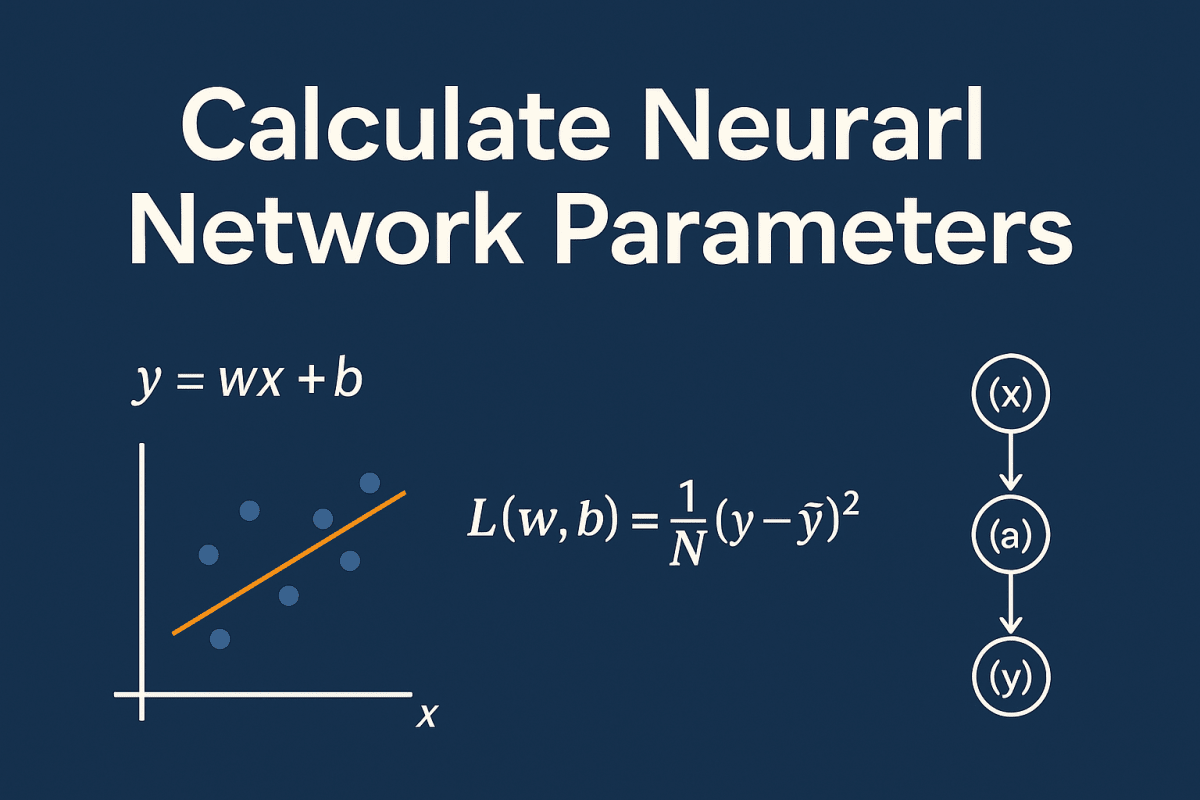
Let's start with a simple linear function:
y = wx + bQ: What's a good w and b?
A: A good set of parameters produces predictions that closely match the actual data. In other words, a good w and b minimize the difference between predicted and real values.
Q: What is a good fit?
A:
- Good fit: The line passes through or near all data points.
- Bad fit: The line is far from many data points.
Q: How can we express this intuition mathematically?
A: For each data point, we calculate the vertical distance between the real value (y) and the predicted value (ŷ). This distance is the error: |y - ŷ|.
To evaluate overall fit, we sum up all these errors: Σ|y - ŷ|. This gives us a total error, which we refer to as the loss function.
Instead of using the absolute value, we square the error for smoother optimization and to emphasize larger mistakes:
L = Σ (yᵢ - ŷᵢ)²To normalize across different sample sizes, we take the average:
L = (1/N) Σ (yᵢ - ŷᵢ)²This is known as the Mean Squared Error (MSE):
L(w,b) = (1/N) Σ (yᵢ - ŷᵢ)²Given data: (x₁, y₁), (x₂, y₂), ..., (xₙ, yₙ)
Linear model: y = wx + b
Loss function: L(w,b) = (1/N) Σ (yᵢ - ŷᵢ)²
Goal: Find the values of w and b that minimize L
Example:
Suppose we have data points: (1,1), (2,2), (3,3), (4,4)
Using y = wx, the loss becomes:
L(w) = (1/4) [(1-1w)² + (2-2w)² + (3-3w)² + (4-4w)²]
Simplifying:
L(w) = (1/4)(30 - 60w + 30w²) = 7.5 - 15w + 7.5w²
Setting derivative to zero gives w = 1 — the best fit line is y = x
Back to Linear Function:
So, for this case, y = x is the best-fit line with minimal loss.
For multivariable functions, we use partial derivatives:
∂L(w,b)/∂w = 0 ∂L(w,b)/∂b = 0This process of finding the best-fit line is known as linear regression.
Gradient Descent:
As w changes, the loss function changes too. We compute the partial derivatives of the loss with respect to w and b, and update them in the opposite direction:
w = w - ∂L(w,b)/∂w
b = b - ∂L(w,b)/∂b
To control the step size, we add a learning rate η:
w = w - η ∂L(w,b)/∂w
b = b - η ∂L(w,b)/∂b
This iterative optimization is called gradient descent.
Neural Network Case:
Now let’s look at a neural network structure:
(x) → (a) → (y)
Input  Hidden  Output

x → g(w₁x + b₁) → a → g(w₂a + b₂) → y → (1/N)Σ(yᵢ - ŷᵢ)² = L

g(z) = 1 / (1 + e^(-z)) (sigmoid)
To compute ∂L/∂w₁, we use the chain rule:
∂L/∂w₁ = ∂L/∂y × ∂y/∂a × ∂a/∂w₁Think of it like gears turning — how much the final output changes with one turn of the input. This is the core idea behind the chain rule from calculus.
We apply this process from output back to input — a technique called backward propagation.
With forward propagation, we compute predictions. With backward propagation, we compute gradients to adjust parameters — this combination powers neural networks.
From simple linear regression to multi-layer neural networks, we've seen how loss functions, gradient descent, and backpropagation help tune models to fit data. But this is just the beginning — many more methods and tricks exist to improve performance, stability, and generalization. Keep exploring, experimenting, and learning — the journey into deep learning is just getting started.