In the previous sections, we saw how matrix operations can be used to calculate neural outputs using linear transformations followed by nonlinear activation functions.
Linear Transformation with Matrix
Suppose we have three inputs: x₁, x₂, and x₃. If there's one output neuron, the function can be represented as:
y₁ = g(W₁x₁ + W₂x₂ + W₃x₃ + b₁)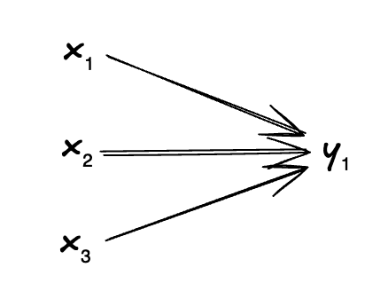
If there's 3 inputs, that is 3W and 3X, and so on.
If there are two output neurons, we simply introduce another function:
y₁ = g(W₁x₁ + W₂x₂ + W₃x₃ + b₁)
y₂ = g(W₁'x₁ + W₂'x₂ + W₃'x₃ + b₂)
This can be represented in matrix form:
Y = g(WX + b)
The layer of neuron did not shown on the formula, what if add more layers to it? We use [l] to denote layers in deep networks:
A[l] = g(W[l]A[l-1] + b[l])
This complex operation is converted into matrix computation, making full use of GPU parallelism to accelerate training and inference in neural networks.
The Problem with Fully Connected Layers
In a fully connected (FC) layer, every neuron is connected to every neuron from the previous layer. While this seems intuitive, it causes inefficiency—especially with image data.
For example, if the input is a 30×30 grayscale image, flattening it creates a vector of 900 values. If the next layer has 1,000 neurons, the FC layer would need 900,000 parameters—very computationally expensive.
Additionally, FC layers ignore the spatial relationships between pixels. This is where convolution comes in.
Introducing Convolution
Instead of flattening, we take a small region of the image—say a 3×3 patch:
162 163 172
169 171 173        // These values are gray values of color
172 174 182
We apply a fixed-size weight matrix (a kernel) to this patch and compute a weighted sum. We repeat this over the image—this is the core of the convolution operation.
The kernel slides over the image to capture local patterns, and the result forms a new matrix (feature map). This reduces the number of parameters and keeps the spatial structure of the image.
From FC to CNN
We can think of replacing FC layers with convolutional layers to both reduce parameters and increase feature extraction. This transition leads us from basic matrix ops to full CNNs.
A common neural network structure looks like this:
Input → Conv → Pool (optional) → FC → OutputThe function becomes:
A[l] = g(W[l] * A[l-1] + b[l])
Pooling layers are often added after convolution to downsample the feature map and retain the most important information with less computation.
Together, these layers—Convolutional, Pooling, and Fully Connected—form what we call a Convolutional Neural Network (CNN), a foundational structure for image recognition tasks.
And that’s a wrap on how we transition from matrix operations to convolutional neural network architectures! I hope you found this post helpful and learned something new along the way.